HNSW:ANN 检索算法(二)
本文介绍的论文是 ANN 检索领域的常见算法 HNSW,原文参见:Efficient and robust approximate nearest neighbor search using Hierarchical Navigable Small World graphs
1 整体介绍
作者是 NSW(Navigable Small World graph)的作者,HNSW 是 Hierarchical NSW 的缩写。如果还不了解 NSW 的,欢迎大家参考我的上一篇文章 NSW:ANN 检索算法(一)。
NSW 有的特征,HNSW 都有。比如 navigable、使用贪心算法等。而 HNSW 在 NSW 的基础上做出的升级是什么呢?
这里补充一下什么是 navigable?比较细致的介绍是:
In graph theory, a navigable graph is one where, starting from any node, you can reach any other node using a greedy algorithm that always chooses the neighbor closest to the target.
上述参见Navigable Graphs for High-Dimensional Nearest Neighbor Search: Constructions and Limits
简单来讲,navigable 就是使用贪心算法,可以从一个节点到另一个节点。虽然这看起来像是废话,但是这在图论中,是一个特别重要的性能,也是作者立论的基础。
第一,Hierarchical,简单来讲就是分层的。不像 NSW,只有一个平面,而 HNSW 是立体的,分了多层的。后面会结合图片来讲到。
第二,性能更优。在低维数据集上,由于 NSW 的多重对数复杂度的缩放,仍然有一个比较严重的性能下降。HNSW 的缩放可以达到对数复杂度。
第三,可以理解为一个概率跳表结构的变种。
2 算法思路
HNSW 算法的思路就是根据链接的长度量级来将其划分到不同的层,并且检索也是在多个层里面进行的。在检索的时候,只有一小部分的链接会用到,和整体的网络量级无关。
检索从最上层开始,(最上层的链接也最长),使用贪心算法遍历,直至找到局部最小值。而后,切换到下一层(链接也比上一层要短些),重复上述过程。参见下图(绿色点是query,红色箭头是贪心算法的检索路径,最上层的红色点是entry point):
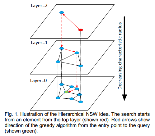
为了保证随机性,HNSW 的构建算法,在插入一个元素之前要进行shuffle。而 HNSW 不同,随机性是通过随机来选择元素所要插入的层来实现的。
3 算法详述
3.1 插入算法
插入算法伪代码见 alg. 1下,对于每一个被插入的元素,它插入的最大层$l$是随机选择的,还有一个指数级下降分布的算法来控制。
插入算法的第一个阶段,即下面第5~7行的内容。从最上层开始,使用贪心算法找到 $q$ 的 $ef$ 个近邻节点。之后,在下一层,使用找到的这几个节点作为起始节点,重复上述过程。找到近邻节点的算法见 alg. 2,它是 NSW 查找算法的一个变种。
插入算法的第二个阶段,即 alg. 1的8~17行。当插入算法遍历的层到了小于等于 $l$ 的时候,第二个阶段和第一阶段的区别是,$ef$ 参数从 $efConstruction$ 变为 1;在每一层找到的近邻节点也和要插入节点产生链接。==注意到,从 $l$ 层到最后一层,每一层都要插入 $q$ 节点。==
在第二阶段选择近邻节点时,有两种方法:第一种方法即 alg. 3,比较直观的算法。第二种算法即 alg. 4,是一种启发式算法。它会扩大候选节点的范围($extendCandidates$),也会裁剪一些节点($keepPrunedConnections$)。具体见算法表述,都是比较简单明了的。
在第二阶段的最后,还会根据传入的每个节点的最大链接数 $M_{max}$ 来进行一个裁剪,即 alg. 1中第14~16行的内容。
\[\begin{aligned} &\textbf{Algorithm 1: INSERT}(hnsw, q, M, M_{\max}, efConstruction, m_L) \\ &\textbf{Input:} \\ &\quad \text{multilayer graph } hnsw, \text{ new element } q, \\ &\quad \text{number of established connections } M, \\ &\quad \text{maximum number of connections } M_{\max}, \\ &\quad \text{size of dynamic candidate list } efConstruction, \\ &\quad \text{normalization factor for level generation } m_L \\ &\textbf{Output:} \\ &\quad \text{update } hnsw \text{ inserting element } q \\ &\quad \\ &1.\ W \leftarrow \varnothing \quad \text{// list for the currently found nearest elements} \\ &2.\ ep \leftarrow \text{get enter point for } hnsw \\ &3.\ L \leftarrow \text{level of } ep \quad \text{// top layer for } hnsw \\ &4.\ l \leftarrow \left\lfloor -\ln(\text{unif}(0..1)) \cdot m_L \right\rfloor \quad \text{// new element's level} \\ &5.\ \textbf{for } l_c \leftarrow L \text{ downto } l+1 \\ &6.\quad W \leftarrow \text{SEARCH-LAYER}(q, ep, ef=1, l_c) \\ &7.\quad ep \leftarrow \text{get the nearest element from } W \text{ to } q \\ &8.\ \textbf{for } l_c \leftarrow \min(L, l) \text{ downto } 0 \\ &9.\quad W \leftarrow \text{SEARCH-LAYER}(q, ep, efConstruction, l_c) \\ &10.\quad \text{neighbors} \leftarrow \text{SELECT-NEIGHBORS}(q, W, M, l_c) \quad \text{// alg. 3 or alg. 4} \\ &11.\quad \text{add bidirectional connections from neighbors to } q \text{ at layer } l_c \\ &12.\quad \textbf{for each } e \in \text{neighbors} \quad \text{// shrink connections if needed} \\ &13.\quad\quad eConn \leftarrow \text{neighbourhood}(e) \text{ at layer } l_c \\ &14.\quad\quad \textbf{if } |eConn| > M_{\max} \quad \text{// shrink connections of } e \\ &15.\quad\quad\quad eNewConn \leftarrow \text{SELECT-NEIGHBORS}(e, eConn, M_{\max}, l_c) \\ &16.\quad\quad\quad \text{set neighbourhood}(e) \text{ at layer } l_c \text{ to } eNewConn \\ &17.\quad ep \leftarrow W \\ &18.\ \textbf{if } l > L \\ &19.\quad \text{set enter point for } hnsw \text{ to } q \end{aligned}\] \[\begin{aligned} &\textbf{Algorithm 2: SEARCH-LAYER}(q, ep, ef, l_c) \\ &\textbf{Input:} \\ &\quad \text{query element } q, \text{ enter points } ep, \\ &\quad \text{number of nearest to } q \text{ elements to return } ef, \\ &\quad \text{layer number } l_c \\ &\textbf{Output:} \\ &\quad ef \text{ closest neighbors to } q \\ &\quad \\ &1.\ v \leftarrow ep \quad \text{// set of visited elements} \\ &2.\ C \leftarrow ep \quad \text{// set of candidates} \\ &3.\ W \leftarrow ep \quad \text{// dynamic list of found nearest neighbors} \\ &4.\ \textbf{while } |C| > 0 \\ &5.\quad c \leftarrow \text{extract nearest element from } C \text{ to } q \\ &6.\quad f \leftarrow \text{get furthest element from } W \text{ to } q \\ &7.\quad \textbf{if } \text{distance}(c, q) > \text{distance}(f, q) \\ &8.\quad\quad \textbf{break} \quad \text{// all elements in } W \text{ are evaluated} \\ &9.\quad \textbf{for each } e \in \text{neighbourhood}(c) \text{ at layer } l_c \quad \text{// update } C \text{ and } W \\ &10.\quad\quad \textbf{if } e \notin v \\ &11.\quad\quad\quad v \leftarrow v \cup e \\ &12.\quad\quad\quad f \leftarrow \text{get furthest element from } W \text{ to } q \\ &13.\quad\quad\quad \textbf{if } \text{distance}(e, q) < \text{distance}(f, q) \text{ or } |W| < ef \\ &14.\quad\quad\quad\quad C \leftarrow C \cup e \\ &15.\quad\quad\quad\quad W \leftarrow W \cup e \\ &16.\quad\quad\quad\quad \textbf{if } |W| > ef \\ &17.\quad\quad\quad\quad\quad \text{remove furthest element from } W \text{ to } q \\ &18.\ \textbf{return } W \end{aligned}\] \[\begin{aligned} &\textbf{Algorithm 3: SELECT-NEIGHBORS-SIMPLE}(q, C, M) \\ &\textbf{Input:} \\ &\quad \text{base element } q, \\ &\quad \text{candidate elements } C, \\ &\quad \text{number of neighbors to return } M \\ &\textbf{Output:} \\ &\quad M \text{ nearest elements to } q \\ &\quad \\ &\text{return } M \text{ nearest elements from } C \text{ to } q \end{aligned}\] \[\begin{aligned} &\textbf{Algorithm 4: SELECT-NEIGHBORS-HEURISTIC}(q, C, M, l, \text{extendCandidates}, \text{keepPrunedConnections}) \\ &\textbf{Input:} \\ &\quad \text{base element } q, \\ &\quad \text{candidate elements } C, \\ &\quad \text{number of neighbors to return } M, \\ &\quad \text{layer number } l, \\ &\quad \text{flag extendCandidates}, \\ &\quad \text{flag keepPrunedConnections} \\ &\textbf{Output:} \\ &\quad M \text{ elements selected by the heuristic} \\ &\quad \\ &1.\ R \leftarrow \varnothing \\ &2.\ W \leftarrow C \quad \text{// working queue for the candidates} \\ &3.\ \textbf{if } \text{extendCandidates} \quad \text{// extend candidates by their neighbors} \\ &4.\quad \textbf{for each } e \in C \\ &5.\quad\quad \textbf{for each } e_{\text{adj}} \in \text{neighbourhood}(e) \text{ at layer } l \\ &6.\quad\quad\quad \textbf{if } e_{\text{adj}} \notin W \\ &7.\quad\quad\quad\quad W \leftarrow W \cup e_{\text{adj}} \\ &8.\ W_d \leftarrow \varnothing \quad \text{// queue for the discarded candidates} \\ &9.\ \textbf{while } |W| > 0 \text{ and } |R| < M \\ &10.\quad e \leftarrow \text{extract nearest element from } W \text{ to } q \\ &11.\quad \textbf{if } e \text{ is closer to } q \text{ than any element in } R \\ &12.\quad\quad R \leftarrow R \cup e \\ &13.\quad \textbf{else} \\ &14.\quad\quad W_d \leftarrow W_d \cup e \\ &15.\ \textbf{if } \text{keepPrunedConnections} \quad \text{// add discarded connections} \\ &16.\quad \textbf{while } |W_d| > 0 \text{ and } |R| < M \\ &17.\quad\quad R \leftarrow R \cup \text{extract nearest element from } W_d \text{ to } q \\ &18.\ \textbf{return } R \end{aligned}\]3.2 检索算法
检索算法如 alg. 5所示。这个算法和当 $l=0$ 时的插入算法很类似。对于插入算法在最后一层返回的做链接的节点,就是检索算法返回的结果。
\[\begin{aligned} &\textbf{Algorithm 5: K-NN-SEARCH}(hnsw, q, K, ef) \\ &\textbf{Input:} \\ &\quad \text{multilayer graph } hnsw, \\ &\quad \text{query element } q, \\ &\quad \text{number of nearest neighbors to return } K, \\ &\quad \text{size of dynamic candidate list } ef \\ &\textbf{Output:} \\ &\quad K \text{ nearest elements to } q \\ &\quad \\ &1.\ W \leftarrow \varnothing \quad \text{// set for current nearest elements} \\ &2.\ ep \leftarrow \text{get enter point for } hnsw \\ &3.\ L \leftarrow \text{level of } ep \quad \text{// top layer for } hnsw \\ &4.\ \textbf{for } l_c \leftarrow L \text{ downto } 1 \\ &5.\quad W \leftarrow \text{SEARCH-LAYER}(q, ep, ef=1, l_c) \\ &6.\quad ep \leftarrow \text{get nearest element from } W \text{ to } q \\ &7.\ W \leftarrow \text{SEARCH-LAYER}(q, ep, ef, l_c=0) \\ &8.\ \textbf{return } K \text{ nearest elements from } W \text{ to } q \end{aligned}\]4 补充材料
如果大家想阅读原论文的话,这里有些背景知识,帮助大家理解。
zoom-in & zoom-out?
”zoom-out“和”zoom-in“类似于显微镜的”粗准焦螺旋“和”细准焦螺旋“,简单理解”zoom-out“就是u粗略地查找,”zoom-in“就是细致地查找。
KNN & ANN?
- KNN:K 近邻查找
- ANN:近似近邻查找